
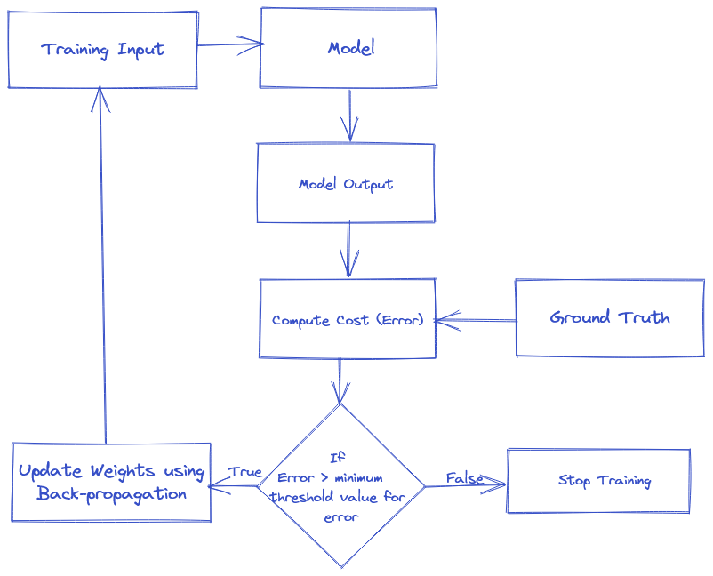
What is Backpropagation?
Backpropagation is a supervised learning algorithm, for training Multi-layer Perceptrons (Artificial Neural Networks).It refers to the method of calculating the gradient of neural network parameters. In short, the method traverses the network in reverse order, from the output to the input layer, according to the chain rule from calculus. It looks for the minimum value of the error function in weight space using a technqiue called the delta rule or gradient descent. The weights that minimize the error function is then considered to be a solution to the learning problem.
Why do we need Backpropagation?
When training a neural network we also assign random values for weights and biases. Therefore, the random weights might not fit the model the best due to which the output of our model may be very different than the actual output. This results in high error values. Thereore, we need to tune those weights so as to reduce the error. To tune the errors we need to guide the model to change the weights such that the error becomes minimum.
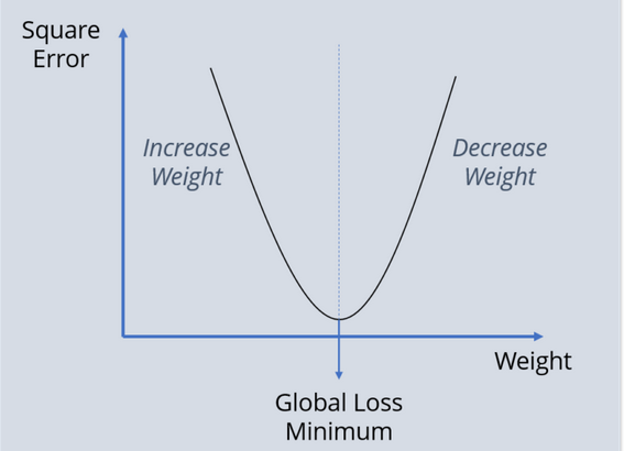 Weights vs Error
Working of Backpropagation
Let’s us consider the Neural Network Below: 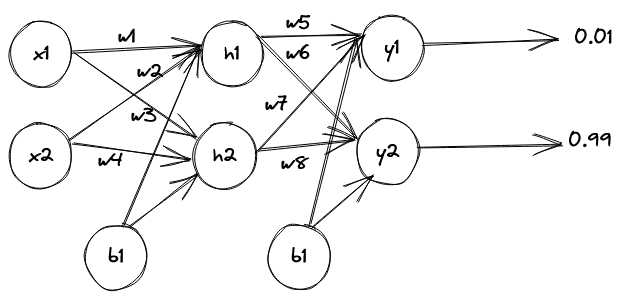
Values: \
- x1= 0.05, x2= 0.10
- b1= 0.35, b2= 0.6
- w1 = 0.15, w2 = 0.20, w3 = 0.25, w4 = 0.30
- w5 = 0.40, w6 = 0.45, w7 = 0.50, w8 =0.55
The above neural network contains the follwowing:
- One Input Layer
- Two Input Neurons
- One Hidden Layer
- Two Hidden Neurons
- One Output Layer
- Two Output Neurons
- Two Biases
Following are the steps for the weight update using Backpropagation:-
Note: We will be using Sigmoid Activation Function.
\(\text{Sigmoid Activation Function}= \frac{1}{1+e^{-x}}\)
- Step 1: Forward Propagation
Net Input for h1:
\(\text{h1} = x1 * w1+x2 * w2+b1\)
\(\text{h1} = 0.05 * 0.15 + 0.10 * 0.20 + 0.35\)
\(\text{h1} = 0.3775\)Output of h1:
\(\text{out h1} =\frac{1}{1+e^{-h1}}\)
\(\text{out h1} = \frac{1}{1+e^{-0.3775}}\)
\(\text{out h1} = 0.5932\)Similary, Output of h2:
\(\text{out h2} = 0.5968\)
Repeat the process for the output layre neurons, using the output from the hidden layer as input for the output neurons.
Input for y1:
\(\text{y1} = \text{out h1} * w5+ \text{out h2} * w6+b2\)
\(\text{y1} = 0.5932 * 0.40 + 0.5968 * 0.45 + 0.6\)
\(\text{y1} = 1.1059\)Output of y1:
\(\text{out y1} =\frac{1}{1+e^{-h1}}\)
\(\text{out y1} = \frac{1}{1+e^{-1.1959}}\)
\(\text{out y1} = 0.7513\)Similary, Output of y2:
\(\text{out y2} = 0.7729\)
Calculating Total Error:
- $E_{total} = E_{1} + E_{2}$
- $E_{total} = \sum_{}^{}\frac{1}{2}(target-output)^{2}$
$E_{total} = \frac{1}{2}(T_{1}-\text{Out y1})^{2}$ + $\frac{1}{2}(T_{2}-\text{Out y2})^{2}$
$E_{total} = \frac{1}{2}(0.01-0.751)^{2}$ + $\frac{1}{2}(0.99-0.772)^{2}$
$E_{total} = 0.29837$
- Step 2: Backward Propagation
Now, we will reduce the error by updating the values weights and biases using back-propagation. To update Weights, let us consider $w5$ for which we will calculate the rate of change of error w.r.t change in weight $w5$
\[\text{Error at w5} = \frac{dE_{total}}{dw5}\]Now,
\[\frac{dE_{total}}{dw5} = \frac{dE_{total}}{\text{douty1}} * \frac{\text{douty1}}{dy1} * \frac{dy1}{dw5}\]Since, we are propagating backwards, first thing we need to do is calculate the change in total errors w.r.t to the output y1 and y2
\[E_{total} = \frac{1}{2}(T_{1}-\text{out y1})^2 + \frac{1}{2}(T_{2}-\text{out y2})^2\] \[\frac{dE_{total}}{d\text{outy1}} = \frac{1}{2} * 2 * (T_{1}-\text{out y1})^{2-1} * (0-1) + 0\] \[\frac{dE_{total}}{d\text{outy1}} = (T_{1}-\text{out y1})* (-1)\] \[\frac{dE_{total}}{d\text{outy1}} = -T_{1}+\text{out y1}\] \[\frac{dE_{total}}{d\text{outy1}} = -0.01 + 0.7513\] \[\frac{dE_{total}}{d\text{outy1}} = 0.7413\]Now, we will propate further backwards and calculate change in output y1 w.r.t its initial input
\[\frac{\text{douty1}}{dy1} = \text{out y1} * (1-\text{out y1})\] \[\frac{\text{douty1}}{dy1} = 0.18681\]Now, we will se how much y1 changes w.r.t change int
\[\frac{dy1}{dw5} = 1 * \text {out h1} * w_{5}^{1-1} + 0 + 0\] \[\frac{dy1}{dw5} = \text {out h1}\] \[\frac{dy1}{dw5} = 0.5932\]w5:
- Step 3: Putting all the values together and calculating the updated weight value.
- Now, putting all the values together:
Now, updating the w5 \(w5 = w5 - \eta * \frac{dE_{total}}{dw5}\)
\[w5 = 0.4 - 0.5 * 0.0821\] \[w5 = 0.3589\]Similarly, we can calculate the other weight values as well
$w6 = 0.4808$
$w7 = 0.5113$
$w8 = 0.0613$
Now, at hidden layer updating w1, w2, w3, and w4:
\[\frac{dE_{total}}{dw1} = \frac{dE_{total}}{\text{dout h1}} * \frac{\text{dout h1}}{dh1} * \frac{dh1}{dw1} \text{ where},\] \[\frac{dE_{total}}{\text{dout h1}} = \frac{dE_{1}}{\text{dout h1}} + \frac{dE_{2}}{\text{dout h1}} \text{ where}\] \[\frac{dE_{1}}{\text{dout h1}} = \frac{dE_{1}}{dy1} * \frac{dy1}{\text{dout h1}} \text{ where}\]\(\frac{dE_{1}}{dy1} = \frac{dE_{1}}{\text{dout y1}} * \frac{\text{dout y1}}{dy1}\)s
\[\frac{dE_{1}}{dy1} = 0.7413 * 0.1868\] \[\frac{dE_{1}}{dy1} = 0.1384\] \[\frac{dy1}{\text{dout h1}} = 0.05539\]Using above values we can calculate the $\frac{dE_{1}}{\text{dout h1}}$ and similarly $\frac{dE_{2}}{\text{dout h2}}$ which in turn can be used to calculate the value of $\frac{dE_{total}}{\text{dout h1}}$. Similarly,calculate the value of $\frac{\text{dout h1}}{dh1}$ and $ \frac{dh1}{dw1}$ to get the change of error w.r.t to change in weight w1. We repeat this process for all the remaining weights.
- After that we will again propagate forward and calculate the output. We will again calculate the error.
- If the error is minimum, we will stop right there, else we will again propagate backwards and upate the weight values.
- This process will keep on repeating until error becomes minimum.
- Now, putting all the values together: