Introduction to Pandas

Getting Started with Pandas

Pandas contains data structures and data manipulation tools designed to make data cleaning and analysis fast and easy in Python.

While pandas adopts many coding idioms from NumPy, the biggest difference is that pandas is designed for working with tabular or heterogeneous data. NumPy, by contract, is best suited for working with homogeneous numerical array data.

import pandas as pd
from pandas import Series, DataFrame
import numpy as np

Introduction to Pandas Data Structures

Series - is a one dimensional array-like object containing a sequence of values and an associated array of data labels, called its index.

obj = pd.Series([4,7,-5,3])

obj
Output: 
    0    4
    1    7
    2   -5
    3    3
    dtype: int64

The string representation of a Series displayed interactively shows the index on the left and the values on the right. Since, we did not specify an index for the data, a default one consisting of the integers 0 through N-1 (where N is the length of the data) is created.

We can get the array representation and index objects of the Sereis via its ‘values’ and ‘index’ attributes respectively.

obj.values
Output: array([ 4,  7, -5,  3], dtype=int64)

obj.index
Output: RangeIndex(start=0, stop=4, step=1)

Often it will be desirable to create a Series with an index identifying each data point

obj2 = pd.Series([4,7,-5,3], index=['d','b','a','c'])
obj2
Output:
    d    4
    b    7
    a   -5
    c    3
    dtype: int64

obj2.index
Output:Index(['d', 'b', 'a', 'c'], dtype='object')

We can use labels in the index when selecting single values or set of values.

obj2['a']
Output: -5

obj2['d']
Output: 4

obj2[['c', 'a', 'd']]
Output:
    c    3
    a   -5
    d    4
    dtype: int64

obj2[obj2 > 0]
Output:
    d    4
    b    7
    c    3
    dtype: int64

obj2 * 2
Output:
    d     8
    b    14
    a   -10
    c     6
    dtype: int64

np.exp(obj2)
Output:
    d      54.598150
    b    1096.633158
    a       0.006738
    c      20.085537
    dtype: float64

Note: Series can also be thought of as a fixed-length, ordered dict, as it is a mapping of index values to data values</p>

'b' in obj2
Output: True

'e' in obj2
Output: False

Converting a Python dict obj to a Series obj in pandas.

sdata = {'Ohio': 35000, 'Texas': 71000, 'Oregon': 16000, 'Utah' : 5000}

obj3 = pd.Series(sdata)

obj3
Output:
    Ohio      35000
    Texas     71000
    Oregon    16000
    Utah       5000
    dtype: int64

When we pass only a dict, the index in the resulting Series will have the dict’s keys in sorted order. We can override this by passing the dict keys in the order we want them to appear in the resulting Series.

type(sdata)
Output:    dict

type(obj3)
Output:    pandas.core.series.Series

states = ['California', 'Ohio', 'Oregon', 'Texas']
obj4 = pd.Series(sdata, index = states)
obj4
Output:
    California        NaN
    Ohio          35000.0
    Oregon        16000.0
    Texas         71000.0
    dtype: float64

Here, 3 values found in sdata were placed in the appropriate locations, but since no value for ‘California’ was found, it appears as NaN(not a number), which is considered in pandas to mark missing or NA values.

pd.isnull(obj4)
Output:
    California     True
    Ohio          False
    Oregon        False
    Texas         False
    dtype: bool

pd.notnull(obj4)
    California    False
    Ohio           True
    Oregon         True
    Texas          True
    dtype: bool

The ‘isnull’ and ‘notnull’ functions in pandas should be used to detect missing data.

obj4.isnull()
Output:
    California     True
    Ohio          False
    Oregon        False
    Texas         False
    dtype: bool

obj3
Output:
    Ohio      35000
    Texas     71000
    Oregon    16000
    Utah       5000
    dtype: int64

obj4
Output:
    California        NaN
    Ohio          35000.0
    Oregon        16000.0
    Texas         71000.0
    dtype: float64

obj3 + obj4
    California         NaN
    Ohio           70000.0
    Oregon         32000.0
    Texas         142000.0
    Utah               NaN
    dtype: float64

Both the Series object itself and its index have a name attribute, which integrates with other key areas of pandas funcitonality:

obj4.name = 'population'

obj4.index.name = 'state'

obj4
Output:
    state
    California        NaN
    Ohio          35000.0
    Oregon        16000.0
    Texas         71000.0
    Name: population, dtype: float64

A series index can be altered in-place by assignment:

obj
Output:
    0    4
    1    7
    2   -5
    3    3
    dtype: int64

obj.index = ['Bob', 'Seteve' ,'Jeff', 'Ryan']

obj
Output:
    Bob       4
    Seteve    7
    Jeff     -5
    Ryan      3
    dtype: int64

DataFrame: A DataFrame represents a rectangular table of data and condains an ordered collection of columns, each of which can be a different value type (numeric, string, boolean, etc.). The DataFrame has both a row and column index; it can be thought of as a dict of Series all sharing the same index.

Note: While a DataFrame is physically two-dimensional, we can use it to represent higher dimensional data in a tabular formati using heirarchial indexing.

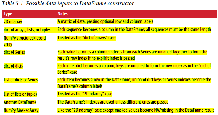
There are many ways to create a DataFrame, though one of the most common is from a dict of equal-length lists or NumPy array:

data = {'state': ['Ohio', 'Ohio', 'Ohio', 'Nevada', 'Nevada', 'Nevada'],
       'year': [2000,2001,2002,2001,2002,2003],
       'pop': [1.5,1.7,3.6,2.4,2.9,3.2]}

frame = pd.DataFrame(data)
frame

Output:

	pop	state	year
0	1.5	Ohio	2000
1	1.7	Ohio	2001
2	3.6	Ohio	2002
3	2.4	Nevada	2001
4	2.9	Nevada	2002
5	3.2	Nevada	2003

For Large DataFrames, the head method selects only the first five rows<

frame.head()

Output:

	pop	state	year
0	1.5	Ohio	2000
1	1.7	Ohio	2001
2	3.6	Ohio	2002
3	2.4	Nevada	2001
4	2.9	Nevada	2002

If we specify a sequence of columns, the DataFrame’s columns will be arranged in that order:

pd.DataFrame(data,columns=['year', 'state', 'pop'])

Output:

	year	state	pop
0	2000	Ohio	1.5
1	2001	Ohio	1.7
2	2002	Ohio	3.6
3	2001	Nevada	2.4
4	2002	Nevada	2.9
5	2003	Nevada	3.2

If passed a column that isn’t contained in the dict, it will appear with the missing values in the result:

frame2 = pd.DataFrame(data, columns = ['year', 'state', 'pop', 'debt'], 
                      index=['one', 'two', 'three', 'four', 'five', 'six'])
frame2

Output:

	year	state	pop	debt
one	2000	Ohio	1.5	NaN
two	2001	Ohio	1.7	NaN
three	2002	Ohio	3.6	NaN
four	2001	Nevada	2.4	NaN
five	2002	Nevada	2.9	NaN
six	2003	Nevada	3.2	NaN

frame2.columns
Output:    Index(['year', 'state', 'pop', 'debt'], dtype='object')

We can retrive a column in a DataFrame as a Series either by dict-like notation or by attribute:

frame2['state']

Output:
    one        Ohio
    two        Ohio
    three      Ohio
    four     Nevada
    five     Nevada
    six      Nevada
    Name: state, dtype: object

frame2.year
Output: 
    one      2000
    two      2001
    three    2002
    four     2001
    five     2002
    six      2003
    Name: year, dtype: int64

Rows can also be retrieved by position or name with the special loc attribute .

frame2

Output:

	year	state	pop	debt
one	2000	Ohio	1.5	NaN
two	2001	Ohio	1.7	NaN
three	2002	Ohio	3.6	NaN
four	2001	Nevada	2.4	NaN
five	2002	Nevada	2.9	NaN
six	2003	Nevada	3.2	NaN

frame2.loc['three']
Output: 
    year     2002
    state    Ohio
    pop       3.6
    debt      NaN
    Name: three, dtype: object

Columns can be modified by assignment. For example, the empty debt column could be assigned a scalar value or an array of values:

frame2['debt'] = 16.5
frame2

Output:

	year	state	pop	debt
one	2000	Ohio	1.5	16.5
two	2001	Ohio	1.7	16.5
three	2002	Ohio	3.6	16.5
four	2001	Nevada	2.4	16.5
five	2002	Nevada	2.9	16.5
six	2003	Nevada	3.2	16.5

frame2['debt'] = np.arange(6.)
frame2

Output:

	year	state	pop	debt
one	2000	Ohio	1.5	0.0
two	2001	Ohio	1.7	1.0
three	2002	Ohio	3.6	2.0
four	2001	Nevada	2.4	3.0
five	2002	Nevada	2.9	4.0
six	2003	Nevada	3.2	5.0

Note: When assigning lists or arrays to a column, we must make sure that the value’s length must match the length of the DataFrame. If we assign a Series, its labels will be realigned exactly to the DataFrame’s index, inserting missing values in any holes

val = pd.Series([-1.2,-1.5,-1.7], index = ['two', 'four', 'five'])

frame2['debt'] = val
frame2

Output:

	year	state	pop	debt
one	2000	Ohio	1.5	NaN
two	2001	Ohio	1.7	-1.2
three	2002	Ohio	3.6	NaN
four	2001	Nevada	2.4	-1.5
five	2002	Nevada	2.9	-1.7
six	2003	Nevada	3.2	NaN

Assinging a column that doesn’t exist will create a new column. And the ‘del’ keyword wil delete columns as with a dict.

frame2['eastern'] = (frame2.state == 'Ohio')
frame2

Output:

	year	state	pop	debt	eastern
one	2000	Ohio	1.5	NaN	True
two	2001	Ohio	1.7	-1.2	True
three	2002	Ohio	3.6	NaN	True
four	2001	Nevada	2.4	-1.5	False
five	2002	Nevada	2.9	-1.7	False
six	2003	Nevada	3.2	NaN	False

del frame2['eastern']
frame2

Output:

	year	state	pop	debt
one	2000	Ohio	1.5	NaN
two	2001	Ohio	1.7	-1.2
three	2002	Ohio	3.6	NaN
four	2001	Nevada	2.4	-1.5
five	2002	Nevada	2.9	-1.7
six	2003	Nevada	3.2	NaN

frame2.columns
Output: Index(['year', 'state', 'pop', 'debt'], dtype='object')

Note: The column returned from indexing a DataFrame is a view on the underlying data, not a copy. Thus, any in-place modifications to the Series will be reflected in the DataFrame. The column can be explicitely copied with the Series’s copy method.

pop = {'Nevada': {2001: 2.4, 2002: 2.9},
      'Ohio':{2000:1.5, 2001: 1.7, 2002: 3.6}}

If the nested dict is passed to the DataFrame, pandas will intrepret the outer dict keys as the columns and the inner dict keys as the rows indices

frame3 = pd.DataFrame(pop)
frame3

Output:

	Nevada	Ohio
2001	2.4	1.7
2002	2.9	3.6
2000	NaN	1.5

We can transpose the DataFrame with similar syntax as in Numpy array. Here, the tranposed dataframe will just be a copy and not a view.

  frame3.T

Output:

	2000	2001	2002
Nevada	NaN	2.4	2.9
Ohio	1.5	1.7	3.6

frame3

Output:

	Nevada	Ohio
2001	2.4	1.7
2002	2.9	3.6
2000	NaN	1.5

The keys in the inner dicts are combined and sorted to form the index in the result. This isn’t true if an explicit index is specified:

pd.DataFrame(pop, index = [2001,2002,2003])

Output:

	Nevada	Ohio
2001	2.4	1.7
2002	2.9	3.6
2003	NaN	NaN

The Dict of Sereis are treated in much the same way

pdata = {'Ohio': frame3['Ohio'][:-1],
        'Nevada':frame3['Nevada'][:2]}
pd.DataFrame(pdata)

Output:

	Nevada	Ohio
2000	NaN	1.5
2001	2.4	1.7

frame3

Output:

	Nevada	Ohio
2001	2.4	1.7
2002	2.9	3.6
2000	NaN	1.5

If a DataFrame’s index and columns have their name attribtues set, these will also be displayed along with the frame

frame3.index.name = 'year'; frame3.columns.name = 'state'
frame3

Output:

state	Nevada	Ohio
year
2000	NaN	1.5
2001	2.4	1.7
2002	2.9	3.6

As with Series, the values attribute returns the data contained in the DataFrame as a two-dimensional ndarray

frame3.values
Output:
    array([[2.4, 1.7],
           [2.9, 3.6],
           [nan, 1.5]])

frame2.values
Output:
    array([[2000, 'Ohio', 1.5, nan],
           [2001, 'Ohio', 1.7, -1.2],
           [2002, 'Ohio', 3.6, nan],
           [2001, 'Nevada', 2.4, -1.5],
           [2002, 'Nevada', 2.9, -1.7],
           [2003, 'Nevada', 3.2, nan]], dtype=object)

Index Objects

Pandas’s Index objects are responsible for holding the axis lables and other metadata. Any array or other sequence of labels we use when constructing a Series or DataFrame is internally convertedto an Index:

obj = pd.Series(range(3), index = ['a','b', 'c'])
index = obj.index
index
Output: Index(['a', 'b', 'c'], dtype='object')

index[1:]
Output: Index(['b', 'c'], dtype='object')

Index objects are IMMUTABLE and thus can’t be modified by the user. Thus makes it safer to share Index objects among data structures.

labels = pd.Index(np.arange(3))

labels
Output: Int64Index([0, 1, 2], dtype='int64')

obj2 = pd.Series([1.5, 2.5, 0],index = labels)

obj2
Output:
    0    1.5
    1    2.5
    2    0.0
    dtype: float64

obj2.index is labels
Output: True

Some users will not often take advantage of the capabilities pro‐ vided by indexes, but because some operations will yield results containing indexed data, it’s important to understand how they work.

frame3

Output:

state	Nevada	Ohio
year
2001	2.4	1.7
2002	2.9	3.6
2000	NaN	1.5

Note: In addition to being array-like, an Index also behaves like a fixed size set

frame3.columns
Output: Index(['Nevada', 'Ohio'], dtype='object', name='state')

'Ohio' in frame3.columns
Output: True

2003 in frame3.index
Output: False

Note: Unlike python sets, a pandas Index can contain duplicate labels

dup_labels  = pd.Index(['foo', 'foo', 'bar', 'bar'])

dup_labels
Output: Index(['foo', 'foo', 'bar', 'bar'], dtype='object')

But selections with duplicate labels will select all occurences of that label.

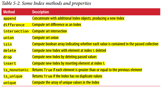
Each Index has a numer of methods and properteis for set logic, which answer other common questions about the data it contains.

Essential Functionality

Reindexing - An important method on pandas objects is reindex, which means to create a new object with the data conformed to a new index.

obj = pd.Series([4.5, 7.2, -5.3, 3.6], index = ['d', 'b', 'a', 'c'])
obj

Output:
    d    4.5
    b    7.2
    a   -5.3
    c    3.6
    dtype: float64

Calling reindex on the above Series rearranges the data according to the new index, introducing missing values if any index values were not already present.

obj2 = obj.reindex(['a', 'b', 'c', 'd', 'e'])
obj2
Output:
    a   -5.3
    b    7.2
    c    3.6
    d    4.5
    e    NaN
    dtype: float64

Note: For ordered data like time series, it may be desirable to do some interpolation or filling of values when reindexing. The method option allows us to do this, using a method such as ffill, which forward-fills the values:

obj3  = pd.Series(['blue', 'purple', 'yellow'], index = [0,2,4])
Output:
    0      blue
    2    purple
    4    yellow
    dtype: object

obj3.reindex(range(6), method = 'ffill')
Output: 
    0      blue
    1      blue
    2    purple
    3    purple
    4    yellow
    5    yellow
    dtype: object

Note: With DataFrame, reindex can alter either the (row) index, columns or both. When passed only a sequence, it reindexed the rows in the result:

frame = pd.DataFrame(np.arange(9).reshape((3,3)),
                    index = ['a', 'c', 'd'],
                    columns = ['Ohio', 'Texas', 'California'])
frame

Output:

	Ohio	Texas	California
a	0	1	2
c	3	4	5
d	6	7	8

frame2 = frame.reindex(['a', 'b', 'c', 'd'])
frame2

Output:

	Ohio	Texas	California
a	0	1	2
b	NaN	NaN	NaN
c	3	4	5
d	6	7	8

The columns can be reindexed with the columns keyword

states = ['Texas', 'Utah', 'California']

frame.reindex(columns=states)

Output:

	Texas	Utah	California
a	1	NaN	2
c	4	NaN	5
d	7	NaN	8

Note: We can reindex more succinctly by lable-indexing withloc, and this way is more preferable by many users.

Dropping Entries from an Axis

Dropping one or more entries from an axis is easy if you already have an index array or list without those entries. As that can require a bit of munging and set logic, the drop method will return a new object with the indicated value or values deleted from an axis:

obj = pd.Series(np.arange(5.), index = ['a', 'b', 'c','d', 'e'])
obj
Output:
    a    0.0
    b    1.0
    c    2.0
    d    3.0
    e    4.0
    dtype: float64

new_obj = obj.drop('c')
new_obj
Output:
    a    0.0
    b    1.0
    d    3.0
    e    4.0
    dtype: float64

obj.drop(['d', 'c'])
Output:
    a    0.0
    b    1.0
    e    4.0
    dtype: float64

With DataFrame, index values can be deleted from either axis.

data = pd.DataFrame(np.arange(16).reshape((4,4)),
                   index = ['Ohio', 'Colorado', 'Utah', 'New York'],
                   columns = ['one', 'two', 'three', 'four'])
data

Output:

	one	two	three	four
Ohio	0	1	2	3
Colorado	4	5	6	7
Utah	8	9	10	11
New York	12	13	14	15

Calling drop with a sequence of lables will drop values from the row labels(axis = 0)

data.drop(['Colorado', 'Ohio'])

Output:

	one	two	three	four
Utah	8	9	10	11
New York	12	13	14	15

We can drop values from the columns by passing axis = 1 or axis = 'columns'

data.drop('two', axis = 1)

Output:

	one	three	four
Ohio	0	2	3
Colorado	4	6	7
Utah	8	10	11
New York	12	14	15

data.drop('three', axis = 'columns')

Output:

	one	two	four
Ohio	0	1	3
Colorado	4	5	7
Utah	8	9	11
New York	12	13	15

Many functions like drop, which modify the size or shape of a Series or DataFrame, can manipulate an object in-place without returning a new object.

obj.drop('c', inplace=True)

obj
Output:
    a    0.0
    b    1.0
    d    3.0
    e    4.0
    dtype: float64

Note: Be careful with the inplace, as it destroys any data that is dropped.

Indexing, Selection, and Filtering

Series indexing (obj[…]) works analogously to NumPy array indexing, except you can use the Series’s index values instead of only integers.

obj = pd.Series(np.arange(4.), index=['a','b', 'c','d'])
obj
Output:
    a    0.0
    b    1.0
    c    2.0
    d    3.0
    dtype: float64

obj['b']
Output: 1.0

obj[2]
Output: 2.0

obj[2:4]
Output:
    c    2.0
    d    3.0
    dtype: float64

obj[['b', 'a', 'd']]
Output:
    b    1.0
    a    0.0
    d    3.0
    dtype: float64

obj[[1,3]]
Output:
    b    1.0
    d    3.0
    dtype: float64

obj[obj<2]
Output:
    a    0.0
    b    1.0
    dtype: float64

Slicing with lables behaves differently than normal Python slicing in that the end-points are inclusive.

obj['b' : 'c']
Output:
    b    1.0
    c    2.0
    dtype: float64

Setting using these methods modifies the corresponding section of the Series

obj['b':'c'] = 5
obj
Output:
    a    0.0
    b    5.0
    c    5.0
    d    3.0
    dtype: float64

Indexing into a DataFrame is for retrieving one or more columns either with a single vlaue or sequence

data = pd.DataFrame(np.arange(16).reshape((4,4)),
                   index = ['Ohio', 'Colorado', 'Utah', 'New York'],
                   columns = ['one', 'two', 'three', 'four'])
data

Output:

	one	two	three	four
Ohio	0	1	2	3
Colorado	4	5	6	7
Utah	8	9	10	11
New York	12	13	14	15

data['two']
Output:
    Ohio         1
    Colorado     5
    Utah         9
    New York    13
    Name: two, dtype: int32

data [['three', 'one']]
Output:
              three   one
    Ohio         1      0
    Colorado     5      4
    Utah         9      8
    New York    13      12
    Name: two, dtype: int32

Indexing like this has a few special cases. First, slicing or selecting data with a boolean array:

data[:2]

Output:

	one	two	three	four
Ohio	0	1	2	3
Colorado	4	5	6	7

data[data['three']>5]

Output:

	one	two	three	four
Ohio	0	1	2	3
Colorado	4	5	6	7
New York	12	13	14	15

The row selection syntax data[:2] is provided as a convenience. Passing a single element or a list to the [] operator selects columns.

Another use case is in indexing with a boolean DataFrame, such as one produced by a scalar comparision

data 

Output:

	one	two	three	four
Ohio	0	1	2	3
Colorado	4	5	6	7
Utah	8	9	10	11
New York	12	13	14	15

data < 5

Output:

	one	two	three	four
Ohio	True	True	True	True
Colorado	True	False	False	False
Utah	False	False	False	False
New York	False	False	False	False

data[data<5] = 0
data

Output:

	one	two	three	four
Ohio	0	0	0	0
Colorado	0	5	6	7
Utah	8	9	10	11
New York	12	13	14	15

This makes DataFrame syntactically more like a two-dimensional NumPy array in this particular case.

Selection with loc and iloc

data

Output:

	one	two	three	four
Ohio	0	0	0	0
Colorado	0	5	6	7
Utah	8	9	10	11
New York	12	13	14	15

The special indexing operators loc and iloc enables us to select a subset of rows and columns from a DataFrame with NumPy-like notation using either axis labels(loc) or integers (iloc)

data.loc['Colorado', ['two', 'three']]
Output:
    two      5
    three    6
    Name: Colorado, dtype: int32

data.iloc[2,[3,0,1]]
Output:
    four    11
    one      8
    two      9
    Name: Utah, dtype: int32

data.iloc[2]
Output:
    one       8
    two       9
    three    10
    four     11
    Name: Utah, dtype: int32

data.iloc[[1,2],[3,0,1]]

Output:

	four	one	tow
Colorado	7	0	5
Utah	11	8	9

Both indexing functions work with slices in addition to single labels or list of labels

data

Output:

	one	two	three	four
Ohio	0	0	0	0
Colorado	0	5	6	7
Utah	8	9	10	11
New York	12	13	14	15

data.loc[:'Utah', 'two']
Output:
    Ohio        0
    Colorado    5
    Utah        9
    Name: two, dtype: int32

data.iloc[:, :3][data['three'] > 5]

Output:

	one	two	three
Colorado	0	5	6
Utah	8	9	10
New York	12	13	14

Integer Indexes

ser = pd.Series(np.arange(3.))
ser
Output:
    0    0.0
    1    1.0
    2    2.0
    dtype: float64

ser2 = pd.Series(np.arange(3.), index = ['a', 'b', 'c'])
ser2
Output:
    a    0.0
    b    1.0
    c    2.0
    dtype: float64

ser2[-1]
Output: 2.0

ser[:1]
Output:
    0    0.0
    dtype: float64

ser.loc[:1]
Output:
    0    0.0
    1    1.0
    dtype: float64

ser.iloc[:1]
Output:
    0    0.0
    dtype: float64

Arithmetic and Data Alignment

An important pandas feature for some applications is the behavior of arithmetic between objects with different indexes. When you are adding together objects, if any index pairs are not the same, the respective index in the result will be the union of the index paris. For users with database experience, this is similar to an automatic Outer Join on the index labels.

s1 = pd.Series([7.3, -2.5, 3.4, 1.5], index = ['a', 'c', 'd', 'e'])

s2 = pd.Series([-2.1, 3.6, -1.5, 4, 3.1], index = ['a', 'c', 'e', 'f', 'g'])

s1
Output:
    a    7.3
    c   -2.5
    d    3.4
    e    1.5
    dtype: float64

s2
Output:
    a   -2.1
    c    3.6
    e   -1.5
    f    4.0
    g    3.1
    dtype: float64

s1 + s2
Output:
    a    5.2
    c    1.1
    d    NaN
    e    0.0
    f    NaN
    g    NaN
    dtype: float64

Here, the internal data alignment introduces missing values in the label locations that don’t overlap. Missing values will then propagate in further arithmetic computations.

In case of DataFrame, alignment is performed on both the rows and the columns

df1 = pd.DataFrame(np.arange(9.).reshape((3,3)),
                  columns = list('bcd'), 
                  index = ['Ohio', 'Texas', 'Colorado'])

df2 = pd.DataFrame(np.arange(12.).reshape((4,3)),
                  columns = list('bde'),
                  index = ['Utah', 'Ohio', 'Texas', 'Oregon'])

df1

Output:

	b	c	d
Ohio	0.0	1.0	2.0
Texas	3.0	4.0	5.0
Colorado	6.0	7.0	8.0

  df2

Output:

	b	d	e
Ohio	0.0	1.0	2.0
Texas	3.0	4.0	5.0
Colorado	6.0	7.0	8.0
Oregon	9.0	10.0	11.0

Adding these together returns a DataFrame whose index and columns are the unionis of the ones in each DataFrame

df1 + df2

Output:

	b	c	d	e
Colorado	NaN	NaN	NaN	NaN
Ohio	3.0	NaN	6.0	NaN
Oregon	NaN	NaN	NaN	NaN
Texas	9.0	NaN	12.0	NaN
Utah	NaN	NaN	NaN	NaN

Since, the ‘c’ and ‘e’ columns are note present in bothe the DataFrame objects, they appears as all missing in the result. The same holds for the ‘Utah’, ‘Colorado’, and ‘Oregon’ whose labels are not common to both objects.

Note: If you add DataFrame objects with no column or row labels in common, then the result will contain all nulls:

df1 = pd.DataFrame({'A': [1,2]})

df2 = pd.DataFrame({'B' : [3,4]})

df1
Output:
    A
  0 1
  1 2

df2
Output:
    B
  0 3
  1 4

df1 - df2
      A   B
  0 NaN NaN
  1 NaN NaN

Arithmetic methods with fill values

In arithmetic operations between differently indexed objects, you might want to fill with a special value, like 0, when an axis lable is found in one object but not the other

df1 = pd.DataFrame(np.arange(12.).reshape((3,4)),
                  columns = list('abcd'))

df2 = pd.DataFrame(np.arange(20.).reshape((4,5)), 
                  columns=list('abcde'))
df2.loc[1, 'b'] = np.nan

df1

Output:

	a	b	c	d
0	0.0	1.0	2.0	3.0
1	4.0	5.0	6.0	7.0
2	8.0	9.0	10.0	11.0

df2

Output:

	a	b	c	d	e
0	0.0	1.0	2.0	3.0	4.0
1	5.0	NaN	7.0	8.0	9.0
2	10.0	11.0	12.0	13.0	14.0
3	15.0	16.0	17.0	18.0	19.0

Adding these together results in NA values in the locations that don’t overlap:

df1 + df2

Output:

	a	b	c	d	e
0	0.0	2.0	4.0	6.0	NaN
1	9.0	NaN	13.0	15.0	NaN
2	18.0	20.0	22.0	24.0	NaN
3	NaN	NaN	NaN	NaN	NaN

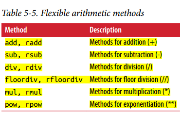
Using the add method on df1,we can pass df2 and an arguemnt to fill_value

df1.add(df2, fill_value = 0)

Output:

	a	b	c	d	e
0	0.0	2.0	4.0	6.0	4.0
1	9.0	5..0	13.0	15.0	9.0
2	18.0	20.0	22.0	24.0	14.0
3	15.0	16.0	17.0	18.0	19.0

df1

Output:

	a	b	c	d
0	0.0	1.0	2.0	3.0
1	4.0	5.0	6.0	7.0
2	8.0	9.0	10.0	11.0

1/df1

Output:

	a	b	c	d
0	inf	1.000000	0.500000	0.333333
1	0.250000	0.200000	0.166667	0.142857
2	0.125000	0.111111	0.100000	0.090909

df1.rdiv(1)

Output:

	a	b	c	d
0	inf	1.000000	0.500000	0.333333
1	0.250000	0.200000	0.166667	0.142857
2	0.125000	0.111111	0.100000	0.090909

When reindxing a Series or DataFrame, we can speciy a different fill value

df1.reindex(columns = df2.columns, fill_value=0)

Output:

	a	b	c	d	e
0	0.0	1.0	2.0	3.0	0
1	4.0	5.0	6.0	7.0	0
2	8.0	9.0	10.0	11.0	0

Operations between DataFrame and Series

arr = np.arange(12.).reshape((3,4))
arr
Output:
    array([[ 0.,  1.,  2.,  3.],
           [ 4.,  5.,  6.,  7.],
           [ 8.,  9., 10., 11.]])

arr[0]
Output: array([0., 1., 2., 3.])

arr - arr[0]
Output:
    array([[0., 0., 0., 0.],
           [4., 4., 4., 4.],
           [8., 8., 8., 8.]])

Here, when we subtract arr[0] from arr, the subtraction is performed once for each row. This is referred to as broadcasting.

frame = pd.DataFrame(np.arange(12.).reshape((4,3)),
                    columns = list('bde'),
                    index = ['Utah', 'Ohio', 'Teas', 'Oregon'])
series = frame.iloc[0]
frame

Output:

	b	d	e
Utah	0.0	1.0	2.0
Ohio	3.0	4.0	5.0
Texas	6.0	7.0	8.0
Oregon	9.0	10.0	11.0

series
Output:
    b    0.0
    d    1.0
    e    2.0
    Name: Utah, dtype: float64

By default, arithmetic between a DataFrame and Series matches the index of the Series on the DataFrame’s columns, broadcasting down the rows

frame - series

Output:

	b	d	e
Utah	0.0	0.0	0.0
Ohio	3.0	3.0	3.0
Texas	6.0	6.0	6.0
Oregon	9.0	9.0	9.0

If an index value is not found in either the DataFrame’s columns or the Series’s index, then the objects will be reindexed to form the union

series2 = pd.Series(range(3), index = ['b', 'e', 'f'])
frame + series2

Output:

	b	d	e	f
Utah	0.0	NaN	3.0	NaN
Ohio	3.0	NaN	6.0	NaN
Texas	6.0	NaN	9.0	NaN
Oregon	9.0	NaN	12.0	NaN

If we want to instead broadcast over the columns, matching on the rows, we have to use one of the arithmetic methods

frame

Output:

	b	d	e
Utah	0.0	1.0	2.0
Ohio	3.0	4.0	5.0
Texas	6.0	7.0	8.0
Oregon	9.0	10.0	11.0

series3 = frame['d']
series3
Output:
    Utah       1.0
    Ohio       4.0
    Teas       7.0
    Oregon    10.0
    Name: d, dtype: float64

frame.sub(series3, axis = 'index')

Output:

	b	d	e
Utah	-1.0	0.0	1.0
Ohio	-1.0	0.0	1.0
Texas	-1.0	0.0	1.0
Oregon	-1.0	0.0	1.0

The axis number that we pass is the axis to mathc on. In this case we mean to match on the DataFrame’s row index (axis=’index’ or axis= 0) and broadcast across the columns.

Function Application and Mapping

Numpy ufuncs (element-wise array methods) also work with pandas objects

frame = pd.DataFrame(np.random.randn(4,3), 
                    columns = list('bde'),
                    index = ['Utah', 'Ohio', 'Texas', 'Oregon'])
frame

Output:
	        b	        d       	e
Utah	-0.059728	-1.671352	-2.322987
Ohio	-1.072084	-1.265158	-1.452127
Texas	-1.487410	-2.289852	-1.427222
Oregon	-0.852068	-0.911926	0.486711

np.abs(frame)
Output:
	        b	        d	        e
Utah	0.059728	1.671352	2.322987
Ohio	1.072084	1.265158	1.452127
Texas	1.487410	2.289852	1.427222
Oregon	0.852068	0.911926	0.486711

Another frequent operation is applying a function on one-dimensional arrays to each column or row. DataFrame’s apply method does exactly this.

f = lambda x: x.max() - x.min()
frame.apply(f)
Output:
    b    1.427681
    d    1.377926
    e    2.809697
    dtype: float64

Here, the function f, which computes the difference between the maximum and minimum of a Series, is invoked once on each column in frame. The result is a Series having the columns of frame as its index.

If we pass axis = 'columns' to apply, the function will be invoked once per row instead

frame.apply(f, axis = 'columns')
Output:
    Utah      2.263259
    Ohio      0.380044
    Texas     0.862630
    Oregon    1.398637
    dtype: float64

Many of the most common array statistics (like sum and mean) are DataFrame methods so using apply is not necessary.

The function passed to apply need not return a scalar value, it can also return a Series with multiple values. For example:

def f(x):
    return pd.Series([x.min(),x.max()],
                    index = ['min', 'max'])
frame.apply(f)

Output:
        b	         d	       e
min	-1.487410	-2.289852	-2.322987
max	-0.059728	-0.911926	0.486711

frame.apply(f, axis = 'columns')

Output:
          min     	max
Utah	-2.322987	-0.059728
Ohio	-1.452127	-1.072084
Texas	-2.289852	-1.427222
Oregon	-0.911926	0.486711

Element wise python functions can be used, too. Suppose, you wanted to compute a formatted string from each floating-point value in frame. You can do this with applymap

format = lambda x: '%2f' % x
frame.applymap(format)

Output:
        b         d         e
Utah	-0.059728	-1.671352	-2.322987
Ohio	-1.072084	-1.265158	-1.452127
Texas	-1.487410	-2.289852	-1.427222
Oregon	-0.852068	-0.911926	0.486711

The reason for the name applymap is that Series has a map method for applying an element-wise function

frame['e'].map(format)
Output:
    Utah      -2.322987
    Ohio      -1.452127
    Texas     -1.427222
    Oregon     0.486711
    Name: e, dtype: object

Sorting and Ranking

Sorting a dataset by some criterion is another important built-in operation. To sort lexicographically by row or column index, use the sort_index method, which returns a new, sorted object

obj = pd.Series(range(4), index = ['d', 'a','b','c'])
obj
Output:
    d    0
    a    1
    b    2
    c    3
    dtype: int64

obj.sort_index()
Output:
    a    1
    b    2
    c    3
    d    0
    dtype: int64

With a DataFrame, we can sort by index on either axis

frame = pd.DataFrame(np.arange(8).reshape((2,4)),
                    index = ['three', 'one'],
                    columns = ['d', 'a', 'b', 'c'])
frame

Output:
	d	a	b	c
three	0	1	2	3
one	4	5	6	7

frame.sort_index()

Output:
	d	a	b	c
one	4	5	6	7
three	0	1	2	3

frame.sort_index(axis = 1)

Output:
	a	b	c	d
three	1	2	3	0
one	5	6	7	4

The data is sorted in ascending order by default, but can be sorted in descending order too using the ascending attribute

frame.sort_index(axis = 1, ascending=False)

Output:
	d	c	b	a
three	0	3	2	1
one	4	7	6	5

To sort a Series by its values, use it’s sort_values method

obj = pd.Series([4,7,-3,2])
obj.sort_values()
Output:
    2   -3
    3    2
    0    4
    1    7
    dtype: int64

Any missing values are sorted to the end of the Series by default

obj = pd.Series([4, np.nan, 7, np.nan, -3, 2])
obj.sort_values()
Output:
    4   -3.0
    5    2.0
    0    4.0
    2    7.0
    1    NaN
    3    NaN
    dtype: float64

When sorting a DataFrame, we can use the data in one or more columns as the sort keys.To do so, pass one or more columns names to the by option of sort_values

frame = pd.DataFrame({'b': [4,7,-3,2,], 'a': [0,1,0,1]})
frame
Output:
	b	a
0	4	0
1	7	1
2	-3	0
3	2	1

frame.sort_values(by='a')
Output:
	b	a
0	4	0
2	-3	0
1	7	1
3	2	1

To sort by multiple columns, pass a list of name

frame.sort_values(by=['a', 'b'])

Output:
	b	a
2	-3	0
0	4	0
3	2	1
1	7	1

Ranking assigns ranks from one through the number of valid data points in an array. The rank methods for Series and DataFrame are the place to look; by default rank breaks ties by assinging each group the mean rank

obj = pd.Series([7,-5,7,4,2,0,4])
obj.rank()
Output:
    0    6.5
    1    1.0
    2    6.5
    3    4.5
    4    3.0
    5    2.0
    6    4.5
    dtype: float64

Ranks can also be assigned according to the order in which they’re observed in the data

obj.rank(method='first')
Output:
    0    6.0
    1    1.0
    2    7.0
    3    4.0
    4    3.0
    5    2.0
    6    5.0
    dtype: float64

Here, instead of using the average rank 6.5 for the entries 0 and 2, they instead have been set ot 6 and 7 because label 0 precedes label 2 in the data.

We can rank in descending order too

obj
Output:
    0    7
    1   -5
    2    7
    3    4
    4    2
    5    0
    6    4
    dtype: int64

obj.rank(ascending=False, method = 'max')
Output:
    0    2.0
    1    7.0
    2    2.0
    3    4.0
    4    5.0
    5    6.0
    6    4.0
    dtype: float64

DataFrame can compute ranks over the rows or the columns

frame = pd.DataFrame({'b': [4.3, 7, -3,2], 'a': [0,1,0,1],
                     'c': [-2,5,8,-2.5]})
frame

Output:
	b	a	c
0	4.3	0	-2.0
1	7.0	1	5.0
2	-3.0	0	8.0
3	2.0	1	-2.5

frame.rank(axis='columns')

Output:
	b	a	c
0	3.0	2.0	1.0
1	3.0	1.0	2.0
2	1.0	2.0	3.0
3	3.0	2.0	1.0

Axis Indexes with Duplicate Labels

obj = pd.Series(range(5), index = ['a', 'a', 'b','b', 'c'])
obj
Output:
    a    0
    a    1
    b    2
    b    3
    c    4
    dtype: int64

The index’s is_unique property can tell you whether its labels are unique or not

obj.index.is_unique
Output: False

Data Selection is one of the main things that behaves differently with duplicates. Indexing a label with multiple entries returns a Series, while single entries return a scalar value.

obj['a']
Output:
    a    0
    a    1
    dtype: int64

obj['c']
Output: 4

This can make our code more complicated as the output type from indexing can vary based on whether a label is repeated or not.

df = pd.DataFrame(np.random.randn(4,3), 
                 index = ['a', 'a', 'b', 'b'])
df

Output:
	0	1	2
a	-0.088814	-0.602398	0.402683
a	1.195694	-0.383322	0.330696
b	-3.542210	0.460190	0.339993
b	-0.718968	-0.049578	0.127387

df.index.is_unique
Output: False

df.loc['b']
Output:
	0	1	2
b	-3.542210	0.460190	0.339993
b	-0.718968	-0.049578	0.127387

Summarizing and Computing Descriptive Statistics

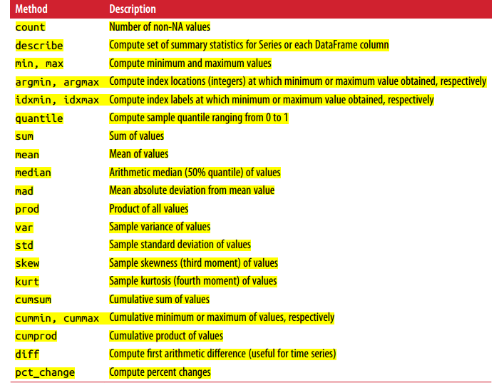
pandas objects are equipped with a set of common mathematical and statistical meth‐ ods. Most of these fall into the category of reductions or summary statistics, methods that extract a single value (like the sum or mean) from a Series or a Series of values from the rows or columns of a DataFrame.

df = pd.DataFrame([[1.4, np.nan], [7.1, -4.5],
                  [np.nan, np.nan], [0.75, -1.3]],
                 index = ['a', 'b', 'c', 'd'],
                 columns = ['one', 'two'])
df

Output:
	one	two
a	1.40	NaN
b	7.10	-4.5
c	NaN	NaN
d	0.75	-1.3

Calling DataFrame’s sum method returns a Series containing Column Sums

df.sum()
Output:
    one    9.25
    two   -5.80
    dtype: float64

Passing axis = 'columns' or axis = 1 sums across the columsn instead

df.sum(axis='columns')
Output:
    a    1.40
    b    2.60
    c    0.00
    d   -0.55
    dtype: float64

df.sum(axis='columns',skipna=False)
Output:
    a     NaN
    b    2.60
    c     NaN
    d   -0.55
    dtype: float64

NA values are excluded unless the entire slice (row or column in this case) is NA. This can be disabled with the skipna option

df.mean(axis='columns', skipna= False)
Output:
    a      NaN
    b    1.300
    c      NaN
    d   -0.275
    dtype: float64

Some methods like idxmin and idxmax return indirect statistics like the index value where the minimum or maximum values are attained:

df.idxmax()
Output:
    one    b
    two    d
    dtype: object

Other methods are accumulations

df.cumsum()

Output:
	one	two
a	1.40	NaN
b	8.50	-4.5
c	NaN	NaN
d	9.25	-5.8

Another type of method is neither a reduction nor an accumulatoin. describeis one such example, producing multiple summary statistics in one shot.

df.describe()

Output:
	one	two
count	3.000000	2.000000
mean	3.083333	-2.900000
std	3.493685	2.262742
min	0.750000	-4.500000
25%	1.075000	-3.700000
50%	1.400000	-2.900000
75%	4.250000	-2.100000
max	7.100000	-1.300000

On non-numeric data, describe produces alternative summary statistics

obj = pd.Series(['a', 'a', 'b', 'c'] * 4)

obj.describe()
Output:
    count     16
    unique     3
    top        a
    freq       8
    dtype: object

Unique Values, Value Counts, and Membership

obj = pd.Series(['c', 'a', 'd', 'a', 'a', 'b', 'b', 'c', 'c'])
uniques = obj.unique()
uniques
Output:    array(['c', 'a', 'd', 'b'], dtype=object)

The unique values are not necessarily returned in sorted order, but could be sorted after the fact if needed (uniques.sort()). Relatedly, value_counts computes a Series containing value frequencies

obj.value_counts()
Output:
    a    3
    c    3
    b    2
    d    1
    dtype: int64

The Series is sorted by value in descending order as a convenience. But it can be sorted in ascending order as well by setting the attribute of sort value to False

pd.value_counts(obj.values, sort = False)
Output:
    a    3
    d    1
    c    3
    b    2
    dtype: int64

isin performs a vectorized set memebership check and can be useful in filtering a dataset down to a subset of values in a Series or column in a Dataframe

obj
Output:
    0    c
    1    a
    2    d
    3    a
    4    a
    5    b
    6    b
    7    c
    8    c
    dtype: object

mask = obj.isin(['b', 'c'])
mask
Output:
    0     True
    1    False
    2    False
    3    False
    4    False
    5     True
    6     True
    7     True
    8     True
    dtype: bool

#equivalent numpy expression
np.in1d(obj,['b','c'])
Output
    array([ True, False, False, False, False,  True,  True,  True,  True])

obj[mask]
Output:
    0    c
    5    b
    6    b
    7    c
    8    c
    dtype: object

Related to isin is the Index.get_indexer method, which gives us an index array from an array of possibly non-distinct values into another array of distinct values

to_match = pd.Series(['c', 'a', 'b', 'b', 'c', 'a'])
unique_vals = pd.Series(['c', 'b', 'a'])
pd.Index(unique_vals).get_indexer(to_match)
Output: array([0, 2, 1, 1, 0, 2], dtype=int64)

In some cases, we may want to compute a histogram on multiple related columns in a DataFrame.

data = pd.DataFrame({'Qu1': [1,3,4,3,4],
                    'Qu2': [2,3,1,2,3],
                    'Qu3': [1,5,2,4,4]})
data
Output: 
	Qu1	Qu2	Qu3
0	1	2	1
1	3	3	5
2	4	1	2
3	3	2	4
4	4	3	4

data.apply(pd.value_counts)
Output:
	Qu1	Qu2	Qu3
1	1.0	1.0	1.0
2	NaN	2.0	1.0
3	2.0	2.0	NaN
4	2.0	NaN	2.0
5	NaN	NaN	1.0

result = data.apply(pd.value_counts).fillna(0)
result

Output:
	Qu1	Qu2	Qu3
1	1.0	1.0	1.0
2	0.0	2.0	1.0
3	2.0	2.0	0.0
4	2.0	0.0	2.0
5	0.0	0.0	1.0